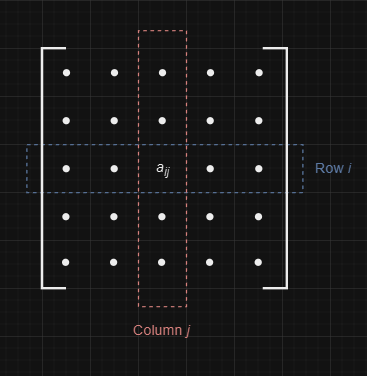
A matrix is a two-dimensional array that contains the same elements as the vector. A matrix can have m rows and n columns. If it does, it is called an m x n matrix. Consider the matrix A below.
\(A =
\begin{pmatrix}
a_{11} & a_{12} & a_{13} & \cdots & a_{1n} \\
a_{21} & a_{22} & a_{23} & \cdots & a_{2n} \\
a_{31} & a_{32} & a_{33} & \cdots & a_{3n} \\
\vdots & \vdots & \vdots & \ddots & \vdots \\
a_{m1} & a_{m2} & a_{m3} & \cdots & a_{mn}
\end{pmatrix}
\)
Each element aij in the matrix is a numerical value displayed in row i and column j.
To add a matrix to another, the matrices must be of the same dimensions, and the elements need to be added to the correct corresponding index.
Consider again the matrix A.
\(A =
\begin{pmatrix}
a_{11} & a_{12} & a_{13} & \cdots & a_{1n} \\
a_{21} & a_{22} & a_{23} & \cdots & a_{2n} \\
a_{31} & a_{32} & a_{33} & \cdots & a_{3n} \\
\vdots & \vdots & \vdots & \ddots & \vdots \\
a_{m1} & a_{m2} & a_{m3} & \cdots & a_{mn}
\end{pmatrix}
\)
The dimensions of matrix A are mxn, meaning that the matrix has m rows and n columns. Matrix A, therefore, can only be added to another matrix with m rows and n columns.
For example:
\(B =
\begin{pmatrix}
b_{11} & b_{12} & b_{13} & \cdots & b_{1n} \\
b_{21} & b_{22} & b_{23} & \cdots & b_{2n} \\
b_{31} & b_{32} & b_{33} & \cdots & b_{3n} \\
\vdots & \vdots & \vdots & \ddots & \vdots \\
b_{m1} & b_{m2} & b_{m3} & \cdots & b_{mn}
\end{pmatrix}\)
The addition is simple, provided that the dimensions match. Add element aij in A to the corresponding element bij in B.
\(A + B =
\begin{pmatrix}
a_{11} & a_{12} & \cdots & a_{1n} \\
a_{21} & a_{22} & \cdots & a_{2n} \\
\vdots & \vdots & \ddots & \vdots \\
a_{m1} & a_{m2} & \cdots & a_{mn}
\end{pmatrix}
+
\begin{pmatrix}
b_{11} & b_{12} & \cdots & b_{1n} \\
b_{21} & b_{22} & \cdots & b_{2n} \\
\vdots & \vdots & \ddots & \vdots \\
b_{m1} & b_{m2} & \cdots & b_{mn}
\end{pmatrix}
\)
\(A + B =
\begin{pmatrix}
a_{11} + b_{11} & a_{12} + b_{12} & \cdots & a_{1n} + b_{1n} \\
a_{21} + b_{21} & a_{22} + b_{22} & \cdots & a_{2n} + b_{2n} \\
\vdots & \vdots & \ddots & \vdots \\
a_{m1} + b_{m1} & a_{m2} + b_{m2} & \cdots & a_{mn} + b_{mn}
\end{pmatrix}
\)
Below is an example of D = A + B - C, where all matrices are of the same dimension.
\(A =
\begin{pmatrix}
1 & 2 & 3 \\
4 & 5 & 6 \\
7 & 8 & 9
\end{pmatrix},
\quad
B =
\begin{pmatrix}
9 & 8 & 7 \\
6 & 5 & 4 \\
3 & 2 & 1
\end{pmatrix},
\quad
C =
\begin{pmatrix}
2 & 3 & 1 \\
5 & 4 & 6 \\
8 & 7 & 9
\end{pmatrix}\)
\(A + B - C =
\begin{pmatrix}
1+9-2 & 2+8-3 & 3+7-1 \\
4+6-5 & 5+5-4 & 6+4-6 \\
7+3-8 & 8+2-7 & 9+1-9
\end{pmatrix} = D\)
\(D =
\begin{pmatrix}
8 & 7 & 9 \\
5 & 6 & 4 \\
2 & 3 & 1
\end{pmatrix}\)
If i = 2 and j = 3, then:
\(Dij = Aij + Bij = Cij\)
Which is:
That equates to:
When multiplying a matrix by a scalar, the dimensions and indices need not be verified. Each element of the matrix is simply multiplied by the scalar.
For example:
\(\alpha \cdot A = \alpha \cdot
\begin{pmatrix}
a_{11} & a_{12} & a_{13} \\
a_{21} & a_{22} & a_{23} \\
a_{31} & a_{32} & a_{33}
\end{pmatrix}
=
\begin{pmatrix}
\alpha \cdot a_{11} & \alpha \cdot a_{12} & \alpha \cdot a_{13} \\
\alpha \cdot a_{21} & \alpha \cdot a_{22} & \alpha \cdot a_{23} \\
\alpha \cdot a_{31} & \alpha \cdot a_{32} & \alpha \cdot a_{33}
\end{pmatrix}
\)
Where every element of the matrix A is multiplied by the scalar α.
Using real numbers, this could be:
\(3 \cdot A = 3 \cdot
\begin{pmatrix}
1 & 2 & 3 \\
4 & 5 & 6 \\
7 & 8 & 9
\end{pmatrix}
=
\begin{pmatrix}
3 \cdot 1 & 3 \cdot 2 & 3 \cdot 3 \\
3 \cdot 4 & 3 \cdot 5 & 3 \cdot 6 \\
3 \cdot 7 & 3 \cdot 8 & 3 \cdot 9
\end{pmatrix}
=
\begin{pmatrix}
3 & 6 & 9 \\
12 & 15 & 18 \\
21 & 24 & 27
\end{pmatrix}
\)
Where every element of the matrix A is multiplied by the scalar 3.
When multiplying two matrices, the dimensions must align correctly. Specifically, if you have a matrix A of dimensions m×n and a matrix B of dimensions p × q, multiplication is possible only if n = p. The resulting matrix C=AB will have dimensions m × q.
The most straightforward scenario is multiplying two square matrices of the same dimensions n × n. That is, both matrices have the same number of rows and columns.
\(Let \ A\ and\ B\ be\ two\ matrices:\
A = \begin{pmatrix}
a_{11} & a_{12} & a_{13} \\
a_{21} & a_{22} & a_{23} \\
a_{31} & a_{32} & a_{33}
\end{pmatrix}, \quad
B = \begin{pmatrix}
b_{11} & b_{12} & b_{13} \\
b_{21} & b_{22} & b_{23} \\
b_{31} & b_{32} & b_{33}
\end{pmatrix}\)
\(The\ product\ C = AB\ is:\
C = \begin{pmatrix}
c_{11} & c_{12} & c_{13} \\
c_{21} & c_{22} & c_{23} \\
c_{31} & c_{32} & c_{33}
\end{pmatrix}
= \begin{pmatrix}
a_{11}b_{11} + a_{12}b_{21} + a_{13}b_{31} & a_{11}b_{12} + a_{12}b_{22} + a_{13}b_{32} & a_{11}b_{13} + a_{12}b_{23} + a_{13}b_{33} \\
a_{21}b_{11} + a_{22}b_{21} + a_{23}b_{31} & a_{21}b_{12} + a_{22}b_{22} + a_{23}b_{32} & a_{21}b_{13} + a_{22}b_{23} + a_{23}b_{33} \\
a_{31}b_{11} + a_{32}b_{21} + a_{33}b_{31} & a_{31}b_{12} + a_{32}b_{22} + a_{33}b_{32} & a_{31}b_{13} + a_{32}b_{23} + a_{33}b_{33}
\end{pmatrix}\)
Or to demonstrate with actual numbers:
\(Let\ A\ and\ B\ be\ two\ matrices:\
A = \begin{pmatrix}
1 & 2 & 3 \\
4 & 5 & 6 \\
7 & 8 & 9
\end{pmatrix}, \quad
B = \begin{pmatrix}
9 & 8 & 7 \\
6 & 5 & 4 \\
3 & 2 & 1\end{pmatrix}\)
\(The\ product\ C= AB\ is:
C = \begin{pmatrix}
(1 \times 9 + 2 \times 6 + 3 \times 3) & (1 \times 8 + 2 \times 5 + 3 \times 2) & (1 \times 7 + 2 \times 4 + 3 \times 1) \\
(4 \times 9 + 5 \times 6 + 6 \times 3) & (4 \times 8 + 5 \times 5 + 6 \times 2) & (4 \times 7 + 5 \times 4 + 6 \times 1) \\
(7 \times 9 + 8 \times 6 + 9 \times 3) & (7 \times 8 + 8 \times 5 + 9 \times 2) & (7 \times 7 + 8 \times 4 + 9 \times 1)
\end{pmatrix}\)
\(Simplifying\ the\ above:\
C = \begin{pmatrix}
30 & 24 & 18 \\
84 & 69 & 54 \\
138 & 114 & 90
\end{pmatrix}\)
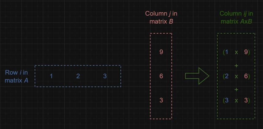
Notice the pattern in finding each element cij in the resulting matrix C = AB: each element cij is calculated by taking the dot product of the i-th row of matrix A and the j-th column of matrix B. Specifically, this involves multiplying each element in the i-th row of A with the corresponding element in the j-th column of B, and then summing these products.
Here is a graphical illustration of this:
These illustrations demonstrate the first row and the first column (Cij):
\(c_{11} = 1 \times 9 + 2 \times 6 + 3 \times 3 = 9 + 12 + 9 = 30
\)
If A is an n×m matrix and B is an m×p matrix, their matrix product AB will be an n×pmatrix. The way this product is calculated is as follows:
Each entry in the resulting matrix AB is obtained by taking the corresponding row from matrix A and the corresponding column from matrix B.
Specifically, you multiply each of the m elements in a row of A with the corresponding m elements in a column of B, and then sum these products. This sum becomes an entry in the matrix AB.
If A is 2×3 (2 rows, 3 columns) and B is 3×2 (3 rows, 2 columns), their product AB will be a 2×2 matrix.
When matrices represent linear transformations (functions that map vectors to other vectors in a linear fashion), the matrix product AB represents the composition of these transformations. This means applying the transformation represented by B first, followed by the transformation represented by A. The resulting transformation is described by the matrix AB.
In essence, matrix multiplication corresponds to performing one transformation after another.
An important observation in matrix algebra is that, in general, matrix multiplication is not commutative. This means that for two matrices A and B, the product A×B does not necessarily equal B×A.
For example, consider matrices A and B as follows:
\(A = \begin{pmatrix}
3 & 1 & 2 \\
-5 & 4 & 1 \\
0 & 3 & -8
\end{pmatrix},\
B = \begin{pmatrix}
0 & 5 & -1 \\
3 & 2 & -1 \\
10 & 0.5 & 4
\end{pmatrix}\)
When C=A×B element c23 in the resulting matrix is:
\(c_{23}^{(A \times B)} = (-5 \times -1) + (4 \times -1) + (1 \times 4) = 5\)
However, if the multiplication is reversed, C=B×A, the element becomes:
\(c_{23}^{(B \times A)} = (3 \times 2) + (2 \times 1) + (-1 \times -8) = 16\)
So, clearly
\(c_{23}^{(A \times B)} \neq\ c_{23}^{(B \times A)}\)
Which means A x B ≠ B = A.
This demonstrates that matrix multiplication is not commutative. This contrasts with scalar multiplication, where the order of multiplication does not affect the result. This non-commutativity is a fundamental characteristic of matrix operations.